With the constant enhancements in cloud capabilities, there really is no excuse for an application to fail because it ran out of resources. In an earlier blog I detailed how to set up autoscaling policies for an application, and today I will detail how to automatically scale entire clusters.
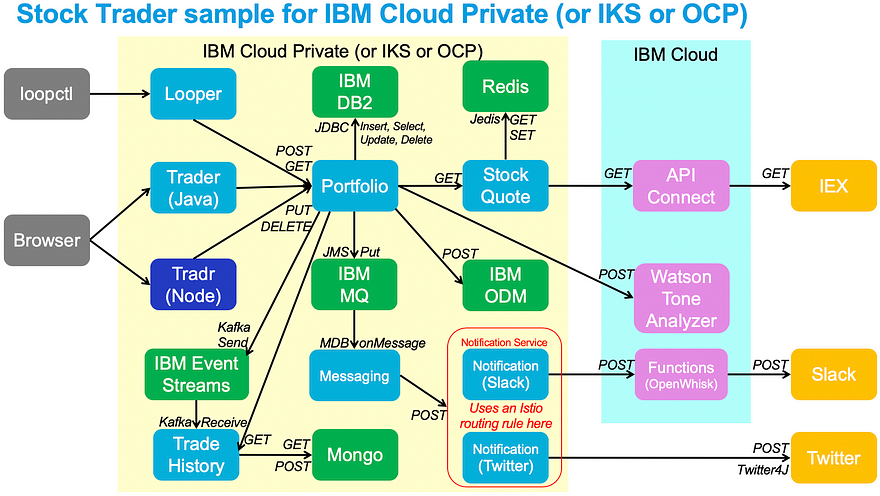
For this procedure, I will be using a Red Hat OpenShift cluster on IBM Cloud running OCP 4.3, and I’ll be using our trusty “Stock Trader” microservices-built application.
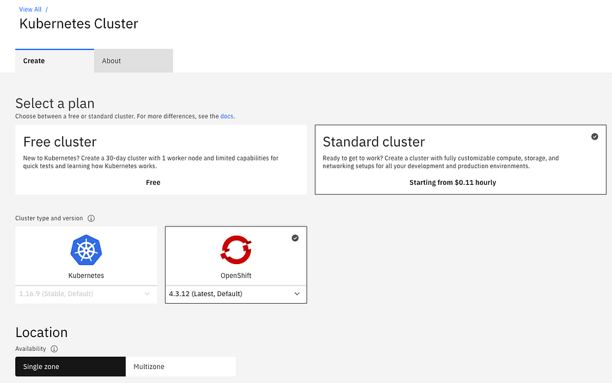
Create Cluster
I first went to IBM Cloud to create a Kubernetes cluster, which I called ‘hintercluster’:
Select type of worker node. I chose 8 vCPU with 32GB RAM
Select number of worker nodes (I chose 3)
That’s it. The IBM service then provisions the worker nodes, prepares them, and in 10 minutes or so I had my cluster ready.
Add Cluster Autoscaler
Once the cluster was created and ready to go, I needed to install the cluster autoscaler (I used this link as my guide). The plug-in is installed through a helm chart so the following steps get helm configured and then the chart installed.
First, I logged into my IBM Cloud account using the ibmcloud command line. Then, I used the oc command line to connect from my laptop to my OpenShift cluster so that the helm commands ran against ‘hintercluster’.
Second, I had to add Helm 3.2 onto my laptop. Since I last used helm in 2.x time, a lot has changed, including the requirement to run the helm tiller on the cluster. This is a great enhancement since I was able to add the helm CLI and start helming without any cluster setup. I did have to alter the written instructions by using brew upgrade helm rather than brew install helm since I had and older release of helm already installed.
brew upgrade helm
Third, I added the chart repo that contained the cluster autoscaler:
When I installed the cluster autoscaler I also needed to define the behavior of it. Notice the — set variable. You will want to use this define your worker node maximum (in this case it is set to 10), and minimum (in this case it is set to 2), and don’t forget to set enabled=true.
To show how the cluster automatically scales in response to applications requesting more resources, I needed to add an application. None better (for us) than using Stock Trader. You can certainly use your own, but this one already had HPAs (Horizontal Pod Autoscalers) defined and it has multiple microservices to scale up and down.
To get Stock Trader installed, I used the new Stock Trader Operator, using this blog entry as a guide.
It was fairly straight forward. I just ran the commands it suggested, and in the UI added the information to our running services for DB2, MQ, Redis, and ODM.
Using the Cluster Autoscaler
Now that we have our application running on our autoscale equipped cluster, I needed to start triggering the cluster autoscaler. The cluster autoscaler scales clusters based on the “resource requests”, or CPU allocation. That means that it will autoscale based on resources requested, not based on actual CPU utilization. In practice the cluster autoscaler will start scaling when a pod cannot be scheduled by the Kubernetes Scheduler due to resource requests not able to be met.
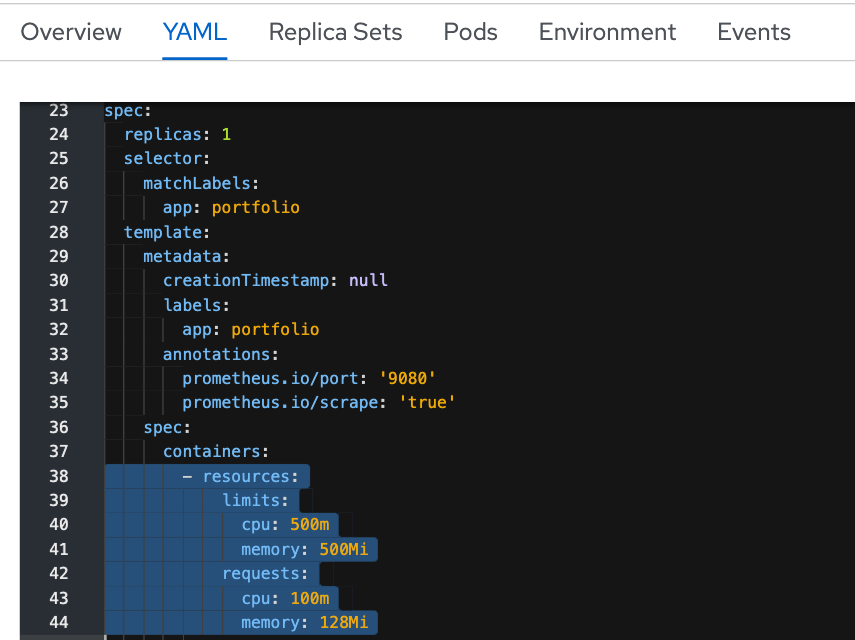
Therefore, to trigger the cluster to start auto-scaling, I added more running pods in the Stock Trader application, and for good measure, also increased the resource requests. To increase resource requests, I clicked on the deployment, then selected the “YAML” tab, and scrolled to the “resources” section:
Since I wanted to ensure the Cluster Autoscaler would trigger, I increased CPU Requests to 1200m. To be clear: an application can be deployed without any resource requests/limits specified, but I do not recommend it. For many reasons (app autoscaling, cluster autoscaling, quota, etc.) you really need to have resource requests/limits specified (along with liveness and readiness probes but you can read about that in our cloud native blogs)
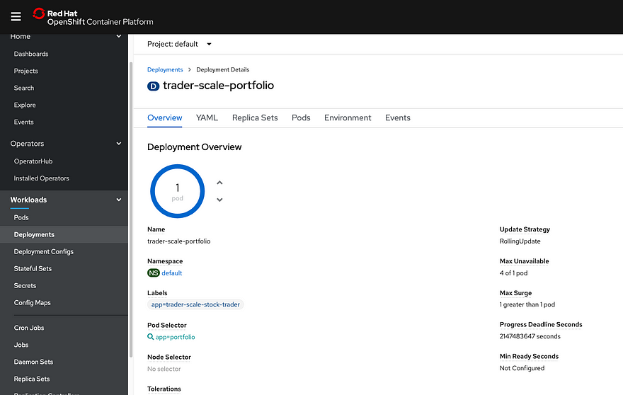
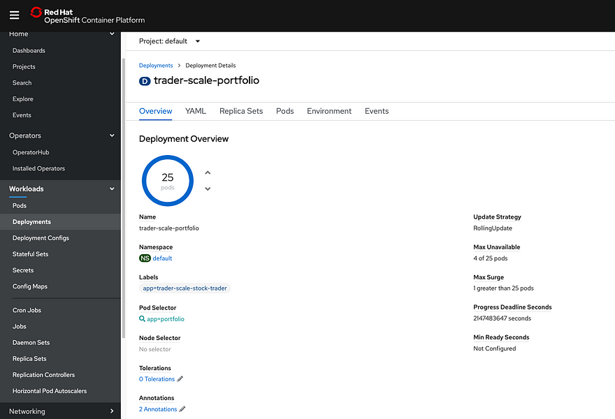
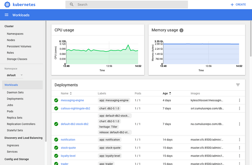
To increase the pod count, I opened the OpenShift UI, navigated to the “trader-scale-portfolio” deployment, and increased the number of pods. It started with one pod, and I scaled it to 25.
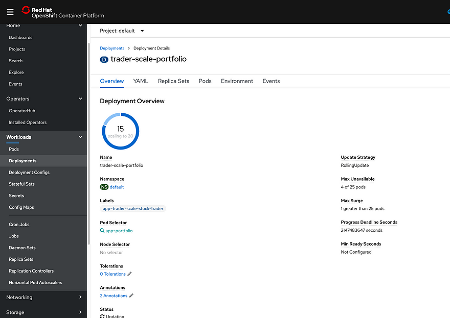
After a few minutes, the deployments stopped, so I looked at the UI and it was paused on 15 deployed pods:
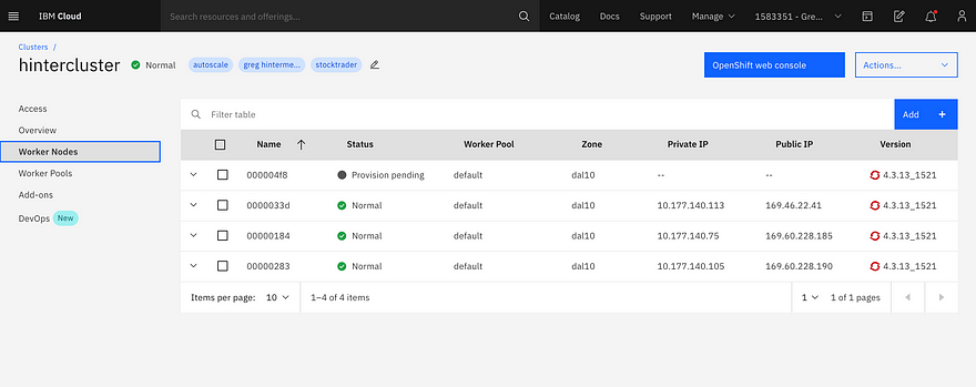
The cluster autoscaler scans the Kubernetes scheduler every 10 seconds, so it will initiate the request fairly quickly to scale-up. Once I noticed the provisioning paused, I then opened the IBM Cloud Clusters UI and saw that the number of worker nodes was being increased:
After a few minutes waiting to provision the VM and prepare it as a worker node, Kubernetes continued to deploy pods. I looked at the deployment UI and soon saw the pod count at 25:
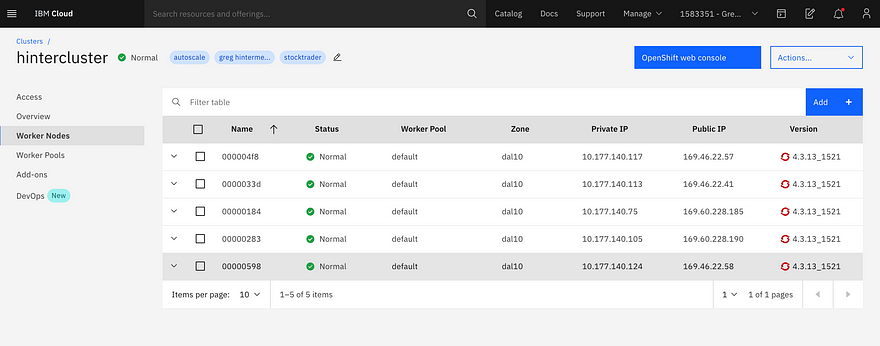
To verify what the cluster autoscaler accomplished, I opened the worker node view and saw the cluster had quickly increased to 5 worker nodes:
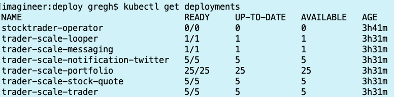
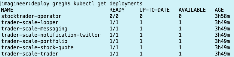
I also ran a check on the command line to ensure all pods were running, I ran
kubectl get deployments
and sure enough, all the deployment scaling increases have completed:
I let the application run for a while, then decided to “scale down” back to 1 pod each microservice. The cluster autoscaler scales down based on there being less than 50% of total CPU being requested, but it waits 10 minutes before removing a compute node, so it takes longer to get to the target “scaled down” state than it does to scale up. That said, the scale down of the pods took merely seconds since it’s just deleting pods. Eventually, everything settled down and I ran the command again to view deployments:
Interesting Findings
One of the interesting findings in this was that the Stock Trader operator quickly proved its worth. In this declarative world of Kubernetes, the operator controls most everything about the Stock Trader application, and as I tried to “mess with the app” in order to test the autoscaling, it kept “fixing” things. For example, I tried to edit the HPA, but the operator wouldn’t let me. Additionally, I tried to manually scale up the deployment (increase the pod count) but it would always kill the newly created pod to match the deployment yaml file. In the end I “scaled down the stock trader operator deployment to zero so that I could temporarily regain control.
What this shows me is that operators are powerful, and that in production they provide an added level of controls so that human error of entering the wrong number can be prevented; but it also shows me that the operator should be installed in a namespace that has stricter access controls than the namespace it’s deployed into. That way only trusted experts can alter the operator itself.
Another interesting finding is that while I started with three worker nodes, and the cluster autoscaler increased to five, when it scaled down, the lowest worker node count was four. Initially I thought there was a defect…and there was! But only in my head! Only later I realized that this is due to the cluster autoscaler using different metrics to scale up vs. scale down. Remember: It uses “Resource Requests” to scale up…if the Kubernetes scheduler can’t provision a pod, it triggers a scale-up. This means the worker node could be at 90% capacity of requested CPU and could still schedule a deployment depending on how big the worker node is and how much resource is requested. However, it will only scale-down if a worker node is running with less than 50% of its total resources available for 10 minutes. This is a fairly big difference. The good news is that these values can be customized. All the details (with sample .yaml) can be found here.
A third interesting finding was that when I edited the YAML to increase resource requests, OpenShift nicely updated the pods based on the deployment strategy, in this case “RollingUpdate”, and used the “MaxUnavailable” value in the deployment. If you look closely at the images above you will see I eventually increased the maximum unavailable to 4 so that the 25 pods would update faster. However, in production, faster is not always better, so think wisely on your update strategy (learn more here)
The last interesting finding is that for an MZR-enabled cluster, which spreads work across three availability zones, the cluster autoscaler will work to scale-up all worker pools of the same type. It may not scale each worker pool for the multi-zone cluster to the same exact number of worker nodes, but will use the same rules to ensure there is capacity to deploy. Alternately, you can choose to opt-out of auto-balancing the matching worker pools resulting in each zone being auto-scaled at its own rate and pace.
For additional deep-dive findings, take a look at this detailed FAQ.
Summary
Scaling clusters, as well as applications, is essential for running mission-critical workloads. The cluster autoscaler works great on both IBM Kubernetes Service and Red Hat OpenShift on IBM Cloud. If you have questions and comments, I’d love to hear of your experiences in the comments.
Application modernization business value can be calculated by measuring the specific impact modernization has on a number of behavioral variables.
Introduction
In working with dozens of clients this past year, we at the Cloud Engagement Hub started refining how we can more quickly help clients calculate the holistic, end-to-end business value of modernizing their applications. What we found is that while past conversations focused on cost savings found on a financial spreadsheet (infrastructure savings, licensing savings, etc), our Cloud Engagement Hub conversations with clients included many other aspects, including development, deployment, and operational behaviors that are altered when an application is modernized. A lot of these aspects can be measured with great accuracy since they are done today in more traditional forms, and equally as measurable after an application is modernized.
The following describes our current progress on how we calculate business value of modernization by measuring (or projecting) changes to many standard variables clients measure every day.
Our goal is to show that working with IBM to modernize applications isn’t a technical experiment, isn’t a science project, but is a solid business decision that will provide a visible return on investment, and will improve revenue in tangible, measurable ways.
Further, by focusing on variables that clients are familiar with, we can set up dashboards to provide real-time weekly progress on the value they are achieving…where based on these facts, can push their teams, or IBM, or both, to achieve the business value they deserve.
As you study this, provide any feedback in the comments. We’d love to discuss this in depth with you.
Variables Used
These are the variables in our pragmatic approach to calculating modernization business value. Each can be measured individually. The idea is that they should be measured before App Mod, and then either projected or measured after App Mod. They should be calculated for the level of modernization you choose: Containerize, Repackage, Refactor, Externalize. Based on your target, the variables will hold different values. The goal is to obtain the change of these variables; the delta. The delta will then be used in the formula to calculate business value.
Note: For some clients, not all variables are relevant. That’s OK. If you don’t have a way to measure, or don’t some of variables will change much when doing App Mod, then leave the change as zero.
Time-Based Behavioral Variables
These time-based variables can be divided into two categories: Development Focused, and Operations Focused. I know…a true DevOps environment doesn’t separate the two, but most enterprise shops are on a transformation journey and many still separate dev and operations.
As will be described in the details section, to calculate these variables, think about the tasks you perform, how many times you do each task, and what it would mean to automate these tasks.
Development Focused:
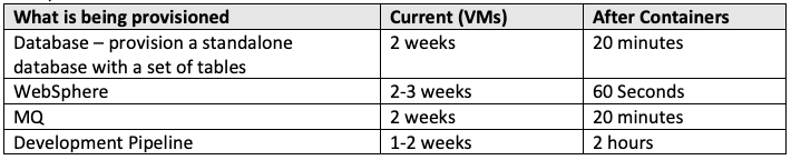
Provisioning (P) Time to stand up dev/test environments (clusters, middleware, pipeline, etc.)
Deployment (D) Time to deploy new app instances on an existing environment for dev/test
Extensibility (E) Time to add new function based on user needs, market changes
Testing (T) Time to test deployable units
Operations Focused:
Provisioning (P) Time to stand up pre-production or production environments (clusters, middleware, pipeline, etc.)
Deployment (D) Time to deploy new app instances on an existing environment for production
Scaling Speed (Ss) Time to scale application to necessary levels to respond to demand
Resiliency (R) Time to recover from a datacenter/environment outage
Maintenance (M) Time to maintain running environments
Time to Market (Tm) Time to deliver new revenue-generating feature to market
Cost Variables
Infrastructure (I) Cost of Infrastructure (VMs, Bare Metal, Kubernetes Clusters) including what’s needed for ‘ready reserve’ for future scaling needs
Labor (La) Cost of labor per unit of measure
License (Li) Cost of licensing for app runtime/middleware
Feature Revenue (Rf) Revenue of a feature / unit of measure
AppMod Cost (Am) Cost to modernize to target level (containerize, repackage, refactor) multiplied by cost per unit of measure
Calculations
To calculate the business value, each element of the equation needs to be measured. Below, the elements represent the changes (delta) of each variable before and after modernization. If you don’t have the “after” measurement, the details section below will offer some suggested defaults based on real client feedback.
Time Saved in Modernization (Vt)
Vt is the aggregated time saved across all time-based variables above. The variables represent the App Lifecycle stages by containerizing, repackaging, or refactoring the application.
Vt = ΔP + ΔD + ΔE + ΔSs + ΔR + ΔM + ΔT
Costs Saved in Modernization (Vc)
Vc is the costs saved based on the time saved that was calculated above. This variable is simple the time saved (Vt) multiplied by labor costs per unit measured.
Vc = Vt · La
Feature Value (Vf)
Vf is the value of delivering a revenue-generating feature earlier due to the time saved modernizing the application. (Feature value) equals the time saved delivering a revenue-generating feature multiplied by revenue per unit measured. This should be run for every feature to reinforce that if a feature can be delivered 6 months early due to modernization, then future delivered features will see that benefit as well. It’s up to each client to determine how many Vf’s should be included into the final business value calculation. Generally, all planned features over the next two years should be used for accurate business value understanding.
Vf1 = ΔTm1 · Rf // Feature one, time saved with modernization, multiplied by estimated revenue of that feature Vf2 = ΔTm2 · Rf // Feature two, time saved with modernization, multiplied by estimated revenue of that feature
Vf3 = ΔTm3 · Rf // Feature three, time saved with modernization, multiplied by estimated revenue of that feature
See the details section below for examples.
Calculate Modernization Business Value Calculate the business value by adding all of the above together, then subtract the cost of modernizing the application itself.
Bv (Business Value) equals the costs saved with modernization (Vc), the infrastructure costs saved (ΔI), the licensing costs saved (Δli), The Feature Value for each planned feature (Vf), and then subtracting the investment to perform the target application modernization techniques (Am)
Bv = Vc + Vf1 + Vf2 + Vf3 + ΔI + ΔLi — Am
One final thought before we move onto the details: Since modernization moves the teams to an agile culture, many of these calculations should have a multiplier to reflect frequency. While teams may provision new environments today only once every 4 months, that may be because its too complicated. If it can be done in 2 hours, then there will be more than 3 provisions per year! There could be 100’s…magnifying the productivity of teams in the new, fully automated, agile culture.
Details: How to Calculate Each Variable
The following sections provide scenarios and suggestions on how we are working to obtain the changes of time due to modernizing the application.
Provisioning (P)
Definition: Time to stand up environments (clusters, middleware, pipeline, etc.)
Scenario: A development team needs an environment to enhance an application with a new feature. They need to stand up an application runtime, Db2, and MQ. This variable will measure how much time it takes from the initial request to when the developer can start working with that environment.
How to get measurements:
Simply asking experienced developers will give you a good estimate
What is being provisioned, and how long does it take before you can use it? (DB, runtime (WebSphere), middleware instances (MQ, IIB, …)
What is it’s purpose (Sandbox, dev, test, prod)
Who needs to approve, authorize, manage the environments?
What automation is used to provision?
It is quite common that a VM will take 2 weeks to become available for developers. While the actual provisioning can be done much more quickly, the approvals, validation, and exceptions result in most provisioning times to be measured in weeks, not hours.
Examples:
For initial estimates, the value of P would equal 6 weeks. If you don’t have an estimate for “After Containers”, then we can use these estimates or values from other client’s experiences we have worked with.
You will notice that you actually have two choices for estimating the delta: 1) effort to accomplish, or 2) linear time to accomplish. In the example above using the low-end estimates (and 8 hours per day), the time saved for provisioning would be as follows:
Before:
Effort to accomplish: 7 weeks (35 days, or 280 hours)
Linear time to accomplish: 3 weeks (15 days, or 120 hours)
After
Time to accomplish: 2:41 hours (assuming some manual authentication)
ΔP = 117.3hours of linear time saved per provisioning instance (even more “effort” saved!)
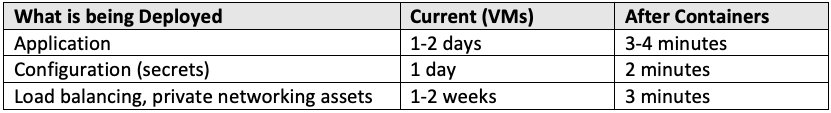
Deployment (D)
Definition: Time to deploy new app instances on an existing environment
Scenario: An application needs to be deployed onto an existing environment. A test team and support education team need to run a new instance of the application. The assumption is that development is complete, and the application components are ready for deployment.
How to get measurements:
Measurements for this can be gathered from asking devs/testers/operations teams
When you get a request to add an application to an existing environment, how long does it take?
What tools do you use to deploy applications?
What configuration is required to connect the application to the dependent resources?
What load balancing and network changes need to happen to get the application running?
In our experience, adding applications to VM-based platforms can take quite some time, whereas a containerized application, using kubectl apply deploy.yaml could take 1–2 minutes.
Examples:
Extensibility (E)
Definition: Time to add new function based on user needs, market changes
Scenario: Product leader defines a new capability to add to an existing application based on user feedback. This variable measures the time it takes to add that capability to a production application.
How to get measurements:
This is intended to measure the productivity of the development team when reacting to a customer request or problem. To get the measurement, it’s important to understand the developer workflow. Some teams may be in a modified waterfall with dependencies and approval boards, while other teams are sprint-based and deliver as soon as the content is ready.
Examples:
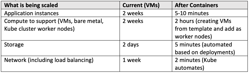
Scaling Speed (Ss)
Definition: Time to scale application to necessary levels to respond to demand
Scenario: As demand increases for an application, it needs to scale up (or down) to meet those demands. Additional compute, storage, networking needs to be added for additional instances. This variable will measure the time it takes to activate that scaling. For WebSphere JavaEE applications, scaling includes acquiring more VMs, add a node to a WAS cell, federate that node, then add a cluster member that lives on that node.
In the end, the expected value will be around what it takes to provision an environment and deploy an application (P + D).
How to get measurements:
This is measured because auto-scaling is not a reality for many applications. “Predictive scaling” is what many application and operations teams perform, predicting the demand, and setting up enough spare capacity to handle that additional demand, well before that demand appears.
To get the measurement, look to past events to see how long it took to set up the compute, storage, network, and application communication so that 3x-50x additional demand could be handled.
Examples:
Resiliency (R)
Definition: Time to recover from a data center/environment outage
Scenario: When an environment (or entire data center) has an outage, applications are obviously impacted, but the impact to end users is what’s most concerning. Current operations teams, regardless of technology used, have a resiliency plan to recover from an outage. Some operations teams go to great lengths to ensure applications running on older technology are resilient. Depending on your situation, you may want to measure a number of activities to come to your Resiliency number.
How to get measurements:
Here are questions you can ask your operations teams:
(Server outage) How much time does it take to recover from a server outage to get the application back to its “normal” state?
(Data Center outage) How much time does it take to recover from a complete data center outage to get the application back to its “normal” state?
There are a number of secondary questions that can add precision to this value. These questions revolve around how much time it takes to prepare an application for an outage so that the time to recover is near zero:
How much time does it take to prepare your application architecture to minimize downtime in the event of an outage?
Are you replicating data to a secondary data center?
Are you keeping the application up to date on a secondary data center?
Are you keeping the that environment hot?
Do you have load balancing that routes to multiple data centers/environments?
How much detection/reaction of an outage is automated?
How much infrastructure is in “ready but idle” state just in case of an outage?
The reality is that after containerizing some applications will still run as “pets” and need application-level synching while others, if architected for cloud, can run as “cattle” and be much more resilient. Either way, running in Kubernetes will automate many of the preparation activities, or at least make them far simpler. (Example: creating a Kubernetes cluster that spans data centers will make worker nodes run in multiple availability zones; greatly increasing application resiliency)
Examples:
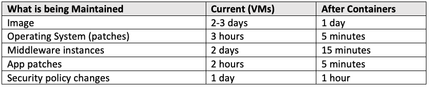
Maintenance (M)
Definition: Time to maintain running environments
Scenario: An application has been running in production, and a variety of issues have been collected ranging from operating system patches, application defects, and middleware patches. The application team needs to maintain the running environment to comply with customer demands, regulations, and security policies.
How to get measurements:
This measurement is all about keeping the environment running properly in leu of patches, found defects, etc. As we all know, with existing VM-based applications (or bare metal), there are VM images to prepare, operating system patches to process, dependent middleware patches to process, application defects to fix and push out into production, changes in security policies to honor, and much more, depending on the application and depending on the company. Here is a list of examples to consider.
Note: The time here does not include development time to code a patch, only the time to push the patch into production.
Examples:
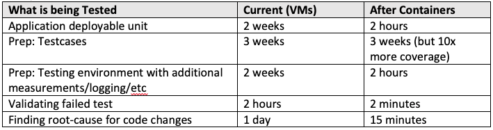
Testing (T)
Definition: Time to test deployable units
In traditional development shops, testing is general a separate activity. The move to cloud-native and a DevOps culture is primarily driven by test-driven development which make testing an embedded and natural element of the DevOps process. However, to get there takes effort and investment. This variable is to measure how long it takes to test an application unit before that unit is deployed into production.
Scenario: A test team receives a deployable unit to test for the next round of application enhancements. They previously provisioned the environment and have provisioned the application. Once testing has completed, the application moves to staging for additional integration testing, and finally to production.
How to get measurements:
This measurement is all about capturing the time it takes to fully test the deployable unit. In traditional cases, the deployable unit is the entire application, but once an app is modernized, the deployable unit is an individual container.
This is also capturing the time it takes to prepare for tests that require real-time feedback. While current platforms like Kubernetes log, monitor, and provide health checks for the container, many traditional environments required user interaction, break points, or exit points to achieve the desired scenario.
As a result, this “Testing” measurement is not only measuring time to test, but time to prepare and maintain the tests and the testing environments.
Examples:
Time to Market (Tm)
Definition: Time to deliver new revenue-generating feature to market
This variable is focused on “If you estimate you can generate $1M of revenue over a year, and by modernizing you can push out the feature 6 months earlier, you can achieve $0.5M in business value in modernizing that application for each revenue-generating feature”.
Scenario: A product team determines a new “visual recognition” system will generate $1M per year in additional revenue for their approval system. The dev team has created sprint plans across 5 dev teams to code necessary changes to the UI, backend, data systems, and new “visual generator” AI algorithms.
How to get measurements:
This measurement can be found by asking an application leader to sketch out this scenario and estimate how long it would take to deliver. Initially they would know “it will take one year”, and those skilled with Kubernetes, DevOps, and cloud-native architecture, could estimate as well “it will take us 6 months”
We also have existing client examples where they saw 30% speed increase.
Examples:
Infrastructure (I)
Definition: Cost of Infrastructure (VMs, Bare Metal, Kubernetes Clusters) including what’s needed for ‘ready reserve’ for future scaling needs
This is a basic measurement of infrastructure costs needed to support the application. No real scenario here is needed, just adding up all the infrastructure needed across Dev, Test, Staging, and Production.
How to get measurements:
Infrastructure costs vary greatly depending on the type of application. For this measurement, keep things simple and ask your IT teams:
How many VMs does it take to run the application across Dev, Test, Staging, and Production?
One recent client we were at counted 23 VMs to run a fairly basic WAS/JavaEE application with the need of multiple environments, and resiliency, and scaling planning.
The “After containers” is a bit trickier. Obviously, it takes VMs to run Kubernetes clusters, so in some cases we bundle the applications to say “while it took 55 VMs to run these eight applications across environments, it only takes 20 VMs to run the same containerized applications across two Kubernetes clusters”. In this case, two clusters because many clients are fine combining Dev/Test/Staging into one cluster, but still want to keep production separate.
Finally, once your count is obtained, find the cost per VM and find the cost of infrastructure.
Examples:
Labor (La)
Definition: Cost of labor per unit of measure
This is a basic measurement of labor costs per day/month/year, based on the unit of measure the time-based calculations were in.
The goal here is to transform the time savings from the first set of variables to a numeric count.
How to get measurements:
List the different roles involved in the time-based calculations and their cost. This will vary based on role and if the labor is contractors or employees.
Also, there is no real “before/after” in this. Developer skills are precious so while some may see as “reducing labor costs” as a downsizing topic, it should be viewed as a way to make your skilled developers more productive.
License (Li)
Definition: Cost of licensing for app runtime/middleware
Modernizing an application can result in reduce licensing costs from a variety of sources, but accuracy in the calculations is essential. For example, some VM hypervisors have a higher licensing cost than others, but the lower licensed hypervisors may have higher support subscriptions.
How to get measurements:
Add up the number of licenses in use on VMs, and then the number of licenses of VMs running in containers.
Feature Revenue (Rf)
Definition: Revenue of a feature / unit of measure
This is an estimate of how much revenue a feature would add over a period of time. This is related to the Time to Market where you can determine “if a feature will bring in an estimated $1M over a year, and I reduce my time to market from 1 year to 6 months, I will have gained $500K in revenue”
Vf (Feature value) = ΔTm · Rf
How to get measurements:
This really comes from the product management team and the market team. This should be known before you are developing a major feature anyway, so should not be a lot of time to calculate.
Here’s what’s important: Even if your team only delivers a subset of the new feature in 6 months, that’s still revenue-generating content out in production faster. Think of it like paying for a loan every week vs. once every 6 months. The sooner you deliver, the more valuable your modernization becomes.
AppMod Cost (Am)
Definition: Cost to modernize to target level (containerize, repackage, refactor) multiplied by cost per unit of measure
This is estimating how much it will take to modernize the target application.
How to get measurements:
The estimating will vary based on the composition and complexity of the application. For JavaEE workloads, using tools like Transformation Advisor will provide a “xyz Developer Days” estimate based on binary scanning of the .ear and .war files. In addition, further analysis of Transformation Advisor’s findings will optimize the estimate to account for duplicate counting, etc.
The final variable should be the number of developer days for an application to be containerized, multiplied by the Labor costs.
Future Variables
There are three other variables to consider, but so far we are not including them because our goal is to focus on variables that can clearly be measured. Scaling Granularity was added as an initial variable, but it overlaps with other variables. One consideration would be to add a “Dependency (Dp)” variable to measure how much time a dev team’s enhancement/patch waits to be deployed so that a dependent team can update their code. Stability (St) is a measurement that we will add later since it will measure how people manually add Istio-like capabilities using traditional networking vs Kubernetes-specific capabilities like Istio.
• Scaling Granularity (Sg) Time to scale smaller components after repackaging apps to smaller, feature-focused containers
• Dependency (Dp) Time waiting for another team to commit their changes before your already-coded changes can be tested/deployed into production.
• Stability (St) Time to write automation to manually create circuit breakers, retry logic, advanced observability (BYO Kubernetes)
Summary
As you can see, while this is still a work in progress, we are quite excited to have the beginning of a framework to measure the business value of Modernization using the behaviors a Dev and Ops team currently uses, with the ability to measure time and cost savings as the application is modernized. To be honest, it’s also exciting to see that when this work progresses, the clients’ culture changes as well to a true DevOps organization…and that’s when savings really accelerate.
We’d love to hear your feedback…see you in the comments!
Last time we walked through the ingredients to add auto-scaling to your containerized applications, and provided a best practice to size your pods, and set resource request and limits. This time we will step through what changes were made to Stock Trader in order to have it automatically scale based on CPU utilization along with liveness and readiness probes.
As a refresher, Stock Trader is our microservices-based application that is freely available on github:
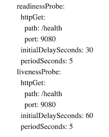
Step 1: Add Readiness and Liveness Probes (see in github)
The readiness and liveness probes we added started with a very basic URL that said “this liberty runtime is up”.
Over time, we added custom probes that were unique for each microservice. As mentioned above, the “Portfolio” microservice was “ready” only when it could connect to its data source. The “Stock-Quote” microservice, however, was only ready when it could connect to the stock quote API provided by API-Connect.
NOTE: as you develop your liveness probe, make sure you have resource limits and a low auto-scale maximum set. In our initial testing, the liveness probe would always fail, which resulted in an immediate restart. However, the HPA declared “I need at least 2 running at average 50% CPU utilization”, and since the startup of a pod took more than 50% CPU, in a very short period of time after we deployed portfolio, we ramped up from 2 pods to 10. It could have easily scaled to 100’s if we had set the maximum that high. Therefore, during these initial stages, we suggest you declare your resource limits, and auto-scale to a small maximum (10, for example).
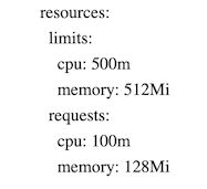
Step 2: Add Resource Requests/Limits
As suggested in the best-practice, if you have a Liberty-based microservice, use the following resources as a starting point:
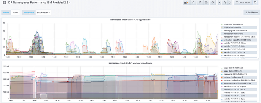
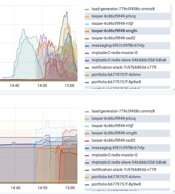
However, as soon as you can, run your microservice with a decent load (simulated if needed) so that you can start graphing your microservice. We used the “ICP Namespace Performance IBM Provided 2.5” Grafana dashboard. This gave us the cleanest example of how our pods ran. If you are using Microclimate, you could also open its “App Monitoring” view and add load onto your Java application.
In this image, we are showing the Stock Trader microservices and we were able to monitor CPU and memory usage in our initial tests:
Once you verify the range of your microservice CPU and memory usage, refine the resource requests and limits.
A couple last notes on resource request/limits:
These resource values are not only critical for auto-scale, they’re also used in basic Kubernetes scheduling. This means that if you specify values that are too high, Kubernetes may not find a worker node with enough resource. We found many times cases where ICP catalog content was sized too high and we could run in development just fine with much less CPU and memory.
Early in development, you may not specify resource requests/limits. For us, this was so that we could have one pod to debug and view logs through. Kubernetes dynamically altered resources for that single pod as long as there was resource available in the compute node. However, we found quickly that as soon as we added resource limits, the pod, during initial testing, could hit resource limits quickly. In summary, as soon as you add resource limits, you will want to create your auto-scale policy to handle additional resource needs.
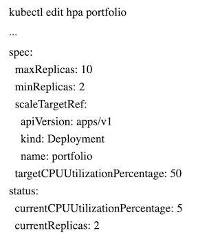
Step 3: Create Auto-scale policies
When first starting out, we recommend creating your first autoscale policy through the CLI. The following example is creating an HPA called “portfolio” to attach to the deployment called portfolio, and manage the number of pods between 2 and 10, based on average CPU % utilization across all “ready” pods so that the average stays around 50%.
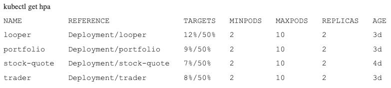
To monitor the hpa, run the following to get the table below:
kubectl get hpa -n stock-trader
Notice in the above output that the “portfolio” HPA requires at least 2 pods to be running and will alter so that the real average CPU % is roughly equal to the target average CPU %. In this case notice that since we do not have any load on the pods, CPU % is only 8%. But since the minimum number of pods is 2, it cannot scale down any further. Once further testing is done, then we added the HPA into the yaml file. Now, every time the “portfolio” microservice is deployed, the associated HPA will also be created.
Step 4: Edit Auto-scale policies
Initially, when we created the HPAs through kubectl, editing was quite messy. As a result, even the docs suggested to delete and recreate the policies. This was simple kubectl delete hpa portfolio. However, we found that after we created the autoscales policies through the deploy.yaml file, editing the HPA through kubectl was easy:
For our Stock Trader microservices we ran a tool we created called “Looper” ( view here). This ran our pods (except the UI) with repeated load. Then, to exercise the UI, we ran a test container:
kubectl run -i — tty load-generator — image=busybox /bin/sh
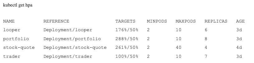
With this load across all microservices, we can now look at the results via the CLI. Viewing realtime HPA details here shows that utilization is too high so the HPA is actively provisioning additional pods:
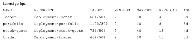
Later on, we see they are more balanced:
Finally, after we stop the load across all pods, the cool-down period of 5–7 minutes results in scaling back to the minimum:
Notice in this Grafana dashboard it shows not only the Stock Trader pods but the looper and load generator pods.
Step 6: Validate Stability
Once your microservices-based app is autoscaling properly, now is the time to run ‘creative tests’, chaos monkey-style tests, to see how it responds to outages and additional load. Here are some examples to try based on Stock Trader architecture:
Add multiple load sources to simulate “Peak usage”
In our case, we needed “Looper” and our UI load generator to generate normal steady-state usage. For additional “peak usage” load, set up a second “looper” running from a different source so that you can hit your application with bursts of activity in addition to the regular load.
Kill pods
Go into the UI or kubectl CLI and just start deleting pods. This will test a real-world scenario where a pod dies and needs to be rescheduled. You could also go into the deployment object and scale up/down manually to see how the HPA reacts.
Taint worker nodes
To simulate pulling the plug on a VM, add a taint to a worker node that prohibits scheduling and execution. This will remove all pods from the VM and schedule them on other worker nodes. In some cases, you won’t have enough resource to auto-scale properly so you can see how your app works in distress.
Remove middleware (Redis)
To simulate a problem with middleware you depend on (Redis, for example), you can scale down to zero the redis deployment. This will then let you validate your code can handle the outage.
Define new data source (test liveness)
Test the liveness check in your pods. If you recall, our “Portfolio” pod said that if it gets three concurrent errors in calling the data source it is no longer “live”. To test this, create a second data source, edit the secret for “portfolio”, and scale down the existing data source (no need to delete … you will be testing this again). You will see the existing portfolio pods get removed after 3 failed attempts at the now-dead data source and when the new pods start, it will pick up the secret with the new (and running) data source and soon enough your app will be alive and kicking.
Step 7: Consider Istio Optimization
For those using Istio for your microservices mesh, the main consideration is the resource requests and limits. During your initial testing with Istio, increase the resource limits for your microservices by 100m CPU and 128Mi Memory so that when the Istio sidecar container is added, your pod will still auto-scale appropriately.
Auto-Scaling using Custom Metrics
If you have custom application-level metrics you want to use in your auto-scaling you can do that by following this documentation. In summary, you will need to install a Prometheus adapter into IBM Cloud Private and then follow the instructions to configure your .yaml files.
OK! Thanks for reading and keep learning! Have questions? I encourage you to post comments below and engage in our conversation.
The promise of Kubernetes with the ability to automatically schedule and scale your application deployments is enticing. But it’s not Magic! Making your microservices-based application automatically scale requires planning by both developers and cloud admins.
The concepts of auto-scaling are not unique to microservices, but what you need to know and understand is different. Developers need to contribute, as well as DevOps engineers, and certainly cloud admins to make auto-scaling successful. Some of that contribution comes by providing liveness and readiness probes in the app configuration, and the rest comes from knowing about the behaviors of each microservice and interactions between microservices.
This blog post will briefly introduce the concept of auto-scaling in Kubernetes. I’ll then follow with part 2, which will provide more concrete insights and supporting examples for specific languages and frameworks.
The following concepts need to be considered when you want to have your application scale in a Kubernetes environment:
Readiness and Liveness probes
Liveness and Readiness probes are essential because they let your microservice communicate to Kubernetes. The Readiness probe tells Kubernetes that the pod is up and ready to receive traffic. The liveness probe tells Kubernetes that the pod is still alive and working as expected.
The trick for the developer is to communicate meaningful status. In our example, if our “portfolio” microservice cannot connect to its data source, then the pod is not ready to receive traffic. The microservice may be up and kicking and in its own world quite healthy. However, since the portfolio microservice depends on the data source to set/get information, it will not want to receive traffic until it has an active data source connection. Once it is “ready”, it then checks for consecutive errors. If portfolio detects three consecutive errors for any communication, then the developer assumes there’s a problem and the pod should be killed and a new one started. Of course, each microservice may require a unique definition of “am I ready” and “am I living”.
Finally, while readiness and liveness probes are not required for auto-scale policies, they are essential so that the pods that are running are productive. Otherwise, the auto-scaler may detect 5 pods running under 50% utilization, but none of them are doing actual work. Timing is important, too. If the “readiness” probe says the pod is “ready” too soon, then work will be routed before the app instance is ready and the transaction will fail. If the “readiness” probe takes too long to say the pod is “ready”, then the existing pods will become overworked and could start failing due to capacity limits.
Readiness and liveness probes are mentioned again because your autoscaling needs to take into account how long it takes for additional pods to become available, and that a liveness probe that is too sensitive can cause your autoscaling to thrash needlessly due to pods being destroyed when they are not truly dead.
Resource requests and limits
Each microservice should specify how much resource (memory and CPU) is required to run. While not required to run in Kubernetes, these resource requests and limits are required for autoscalers to kick in. In Kubernetes, you will want to specify resource requests (how much CPU and Memory to allocate initially when bringing up the pod), and resource limits (the maximum CPU and Memory to allocate over time).
Here’s a sample that a deploy.yaml file would have to specify resource requests and limits:
Horizontal Pod Autoscaler
The Horizontal Pod Autoscaler (HPA) is created by attaching itself to a deployment or other Kube object that controls pod scheduling. In its most basic form, the HPA will look at all pods in a deployment, average the current CPU utilization across all the pods, and if the percent utilized is more than what the HPA is set to, then the HPA will provision additional instances. Conversely, if the percent utilized is less than what the HPA is set to, then the HPA will remove instances until the utilization is approaching what was desired.
Here I’m creating an HPA that attaches itself to the deployment called “portfolio”, and will scale the number of pods between 2 and 10, depending on if the average CPU utilization is above or below 50%.
Vertical Pod Autoscaler
An emerging capability in Kubernetes is vertical pod autoscaling (VPA), which means it can scale the resource requests / limits in real-time so an individual pod can take up more resource.
VPAs can be quite useful for applications that are not written to horizontally auto-scale. If it needs more resource then it can vertically scale. While the best practice is to architect your application for auto-scale, there are some cases where it is not possible and VPA is a good option.
Further, VPAs can be powerful companions to HPAs. For example: If I have an HPA provisioning new pods, it may come up against capacity limits for available worker nodes. In that case, a new pod will not be provisioned. This can happen when the Kubernetes scheduler fails due to affinity rules, resource availability for full pods, readiness probe indicating delay, etc). If you set a VPA to scale the pods vertically in that situation (give each pod 10–20% more CPU and/or Memory), then the existing pods could have some “breathing room” and grow with the small amount of resource still available in the worker node they’re running in.
Node Affinity, Taints and Tolerations
Node affinity, taints and tolerations allow users to constrain which worker nodes an application can be deployed to.
An affinity rule tells Kubernetes what kind of worker node the pod requires or prefers (you can think of it as “hard” or “soft” compliance). The affinity matching is based on node labels. This means that you can prefer that your pod runs on any of the 5 of the 50 worker nodes in the cluster that are labeled as “GPU-enabled”, and also require that the nodes run on any of the 20 of the 50 worker nodes labeled as “Dept42”.
To view the labels on a node, run kubectl get nodes -o wide — show-labels
Taints and Tolerations tell Kubernetes what kind of pods a worker node will accept. This means that a set of worker nodes can be tainted with “old-hardware” and only pods that have a toleration for “old-hardware” will be scheduled.
Think of it this way:
affinity is pod-focused: “I am a pod…there are so many nodes to choose from let me filter so I get one I will run well on”. Affinity lets the pod choose what nodes it will deploy into based on how the nodes are labeled. “I prefer new hardware nodes” “I require GPU-equipped nodes” and then Kubernetes will schedule appropriately.
Taints/Tolerations is node-focused: “I am a worker node…there are so many pods out there, but only certain ones will run well on me due to my unique traits…I will add a taint to require pods to declare that it will tolerate this unique trait”. Taints let the node declare “I am old hardware” or “I am only for production” and as a result, the Kubernetes scheduler will only deploy pods onto those nodes if the pod has a toleration matching that taint: “I am production pod” or, “I will run on old hardware”.
This is one reason why clear communication between development and cloud ops is essential.
Resource Quota
Each namespace in Kubernetes can have a resource quota. This is set up by the cloud admin to limit how much resource can be consumed within a namespace. As this is a hard limit (actual number, not percentage), once an application scales up to the quota limit, it will get a failure if trying to auto-scale beyond the quota.
Further, if a quota is set on a namespace, all pods must have resource requests/limits specified or the scheduling of that pod will fail.
This is yet another reason why clear communication between development and cloud ops is essential.
Other Isolation Policies
IBM Cloud Private has support for many levels of multi-tenancy. This includes the ability to control workload deployments to specific resources like worker nodes, VLANs, network firewalls, and more based on teams and namespaces.
Have I mentioned that your development team needs to have clear communication with your cloud ops team? I think so.
Here is a summary of what you should consider when auto-scaling your application. The actual numbers may vary based on your application, so use this as guide.
As you initially create your microservice, give your resource requests/limits a sensible default. This could vary greatly depending on your base image, runtime, etc. For example, for Liberty runtimes, set it between 200m and 1000m for CPU, and 128Mi and 512Mi to Memory. If you set the limits too low, the autoscaler may trigger an additional instance during initial startup because it’s taking too much CPU.
Run initial unit tests and use Grafana monitoring to see actual CPU and Memory usage during your tests.
Refine your resource requests/limits as needed so your resource limits are 20% more than monitored maximum usage.
Set your initial auto-scale policy to scale your application at 50% of CPU usage.
If you use Istio, increase all resource limits by 100m CPU and 128Mi Memory to handle the additional side-car.
Work with your cloud ops team if any affinity rules or resource quotas will be in place in the clusters across your stages of delivery: development, test, stage, production.
Note: For classic WebSphere applications that you migrated into containers using Transformation Advisor, you may not be able to auto-scale. That said you should still create good liveness and readiness probes and set your resource request/limits.
Next time we will step through how that best practice is set up using Liberty-based microservices.
OK! Thanks for reading and keep on the lookout for Part 2 coming soon!
Part of my work in the Cloud Engagement Hub is to help clients modernize their applications. I’ve spent years focused on public and private cloud environments, and I show, through technical expertise, how clients can modernize their applications through containerizing workloads and running them across public and private clouds. I get quite deep into the technology, use cases, and value of modernizing applications onto a modern cloud-native platform like Kubernetes.
But I have to come clean: To the 100s of clients I’ve presented to, demoed to, had deep-dive analysis with, I have one thing to say:
I apologize.
I apologize, on behalf of our entire industry, for making app modernization appear simplistic…
…for implying that your “Enterprise App” could be treated like an iPhone app…like a cute little rounded square that you could lift, transform, and with a single tap run in a shiny, fancy new cloud environment with all the benefits of cloud, DevOps, security, and infinite scalability.
I know, most of the time we are forced to simplify our conversations to fit within 40 minute technical sessions at conferences, or short client visits, but we both know there’s so much more we should be discussing.
I apologize on behalf of our industry. We are so competitive that we smooth the modernization reality down to a shiny, polished, wooden goblet that only the finest bourbon-barrel stout pours out of, instead of what it is: a heavy, splintered, thorn-laden pile of reclaimed wood that, once you grab as much as you think you can move, scream at uncovering a hornets nest of issues…hidden for years, just waiting to attack any who dare clear away 20 years of undergrowth.
Finally, I apologize for calling these enterprise applications “apps”, instead of what they are: Time-tested enterprise solutions that fueled your company into the enterprise it is today but now suffer from that same span of time where countless enhancements, add-ons, alterations, and “next-gen transformation” projects through the years have resulted in a solution that should be in the “Smithsonian museum of historical app technology”.
The stark reality is that these enterprise applications can no longer sustain the demands of this modern, cloud-centric environment we all live in, and more importantly, meet our customers’ demands. As my new friend Stephanie said, “your enterprise applications have been architected with time; let us modernize them so you can architect them with intent”.
Modernization has to happen, it’s just a matter of how. And while it’s tempting to keep it simple to show our awesomeness, I, and my colleagues, are here to show the full reality of modernization, how we can help you, and yes…to show our awesomeness through actions, not talk.
From here on out, I make the following vow:
I will, through technical evidence, show a realistic modernization journey that your enterprise applications could take. We will have hard conversations about what it means to modernize, migrate, retain, retire, and replace your applications, along with all the middleware, data, security, and storage that goes along with it. We will talk about your cloud landing zones: the pros and cons of each technology; the fact that you will need to spend MORE money to modernize before you see benefits, but that through continuous modernization of your applications, you will see great value on the other side. We will celebrate your modernization success, and then discuss “what happens next”; how your DevOps processes, your culture, your multicloud capabilities, have all changed and will continue to evolve…and that this is just the beginning of your amazing acceleration to awesomeness.
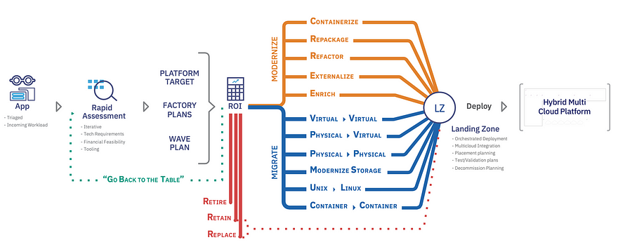
To do that we will look at our Modernization journey map (Figure 1), and we will take your knowledge, add our assessment, plan our attack, and depending on the complexity of your enterprise application, take multiple parallel modernization journeys. Once ready, we will deploy them into the landing zone of your choice so that your business can accelerate.
For example, I know that even the most basic enterprise app (I know, I’m already calling your thorn-laden hornets’ nest of a solution a cute app) will consist of multiple components: a JavaEE runtime and a database, running on either dated VMs or physical servers. I also know that most of your applications are more complex with multiple components ranging from multiple JavaEE runtimes (WebSphere, WebLogic, JBoss, Tomcat), databases, middleware, “helper add-ons” coded in C, C++, and many have core components coded in COBOL running in a mainframe.
Further, I know that due to the increasing speed of development demands outpacing the speed of VM delivery from IT resulted in your VMs becoming “dirty”; filled with extra tools and helper-apps that sometimes are not even related to a single solution. I know that because I did it too. I needed space to run a tool, and since it would take too long to request a new VM, I just picked one that had low utilization. Repeat this over 10 years and you get this gut-punching “very-bad-day” when you realize that even if you modernize the JavaEE app into a containerized workload and run it in Kubernetes, you still can’t decommission the VM because of all the riff-raff still running in that VM.
When we get to work, we will show how modernizing the “basic” enterprise app into a cloud landing zone will require multiple journeys: containerizing the JavaEE component, migrating the database VM, and at least initially, migrating the VM the Java workload was on to keep the helper apps running.
We will talk about deployment patterns the whole app requires, and the characteristics the app components demand (proximity to each other for performance, latency requirements, data requirements, etc ). This will create consistency in how the apps are deployed onto the target cloud, how they are connected, what security policies and isolation policies are used, what quality and type of storage is used, and on and on.
We will talk about how development practices and operations practices all need to modernize along with your apps. It will be hard, filled with fear (and sometimes failure), but changing culture is probably harder than changing technologies (I know, I’ve done it many times). We will start with small successes…MVPs that you find value in…that help in not only starting your app on its modernization journey, but also your developers, operations teams, and how they will merge into a true DevOps culture.
Further, we will discuss that even the term “deploying into the cloud” is simplistic. We know you want to keep your options open, that cost, location (public, private, multiple vendors) cloud region, capabilities, provided services, network and security capabilities, all matter. We will discuss that some of your apps may thrive on one cloud and others may thrive on another. As a result, multi cloud management is a reality. I know that, and you know it, so we might as well talk it through and make it work like you want.
At the end of the day, my goal is to help your business succeed…to thrive so your clients are delighted (I know…not a technical statement, but true none-the-less). If I can help a fellow human succeed, I feel better, and your trust in me grows. I hope you come to realize, at least for me, I’m not here to sell you our products, I’m here to sell you…
Technical Accuracy
…and a relationship you can depend on throughout your modernization journey.
The goal of many enterprise clients is to be able to modernize key applications and run them wherever they want: On a private cloud in their own data center (where their sensitive data lives), on a public cloud (where they get scale, world-wide reach), or even better, on both private and public…where it becomes a true hybrid application taking advantage of the best of both environments.
In late March, IBM shared how clients could run their modernized applications in a hybrid environment across IBM Cloud Private and IBM Cloud Kubernetes Service in IBM Cloud. This essential capability, captured in the following video, showcases how a client can transform their application, where both development teams and cloud ops teams can both be delighted.
Today, I am thrilled to share enhancements that make it even easier to create clusters, manage catalog content, and deploy developed apps across hybrid cloud environments. Specifically, with this latest enhancement of IBM Cloud Private 2.1.0.3, Fix Pack 1, users can extend a new or existing IBM Cloud Private deployment with the following capabilities:
Create additional Kubernetes clusters using a template from IBM Cloud Private
Curate which services developers have access to, and let them provision on either private or public clusters with self-service capability
Deploy a custom app into both private and public environments from the same developer environment
Create additional private and public Kubernetes clusters from your IBM Cloud Private Catalog
The first enhancement is the ability for any authorized user to provision a new IBM Cloud Private cluster or IBM Cloud Kubernetes Service cluster.
For example, once you install IBM Cloud Automation Manager onto your IBM Cloud Private cluster, you can create a brokered service (with customized variables limiting and controlling what options are available) that will let any authorized user create the IBM Cloud Kubernetes Service cluster onto your IBM Cloud account. An optional VPN can be automatically deployed to securely connect the two clusters, if desired.
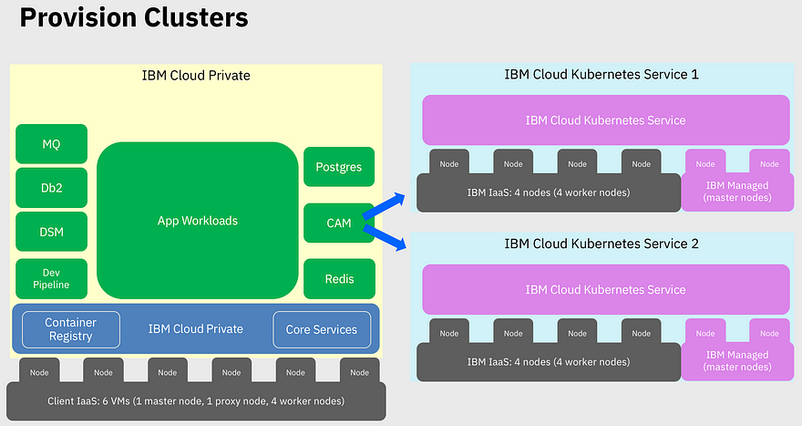
Figure 1: Multiple clusters created from one IBM Cloud Private cluster
Here are the steps you will follow. For each step, I’ve added a link to the Knowledge Center (product documentation) that provides step-by-step instructions.
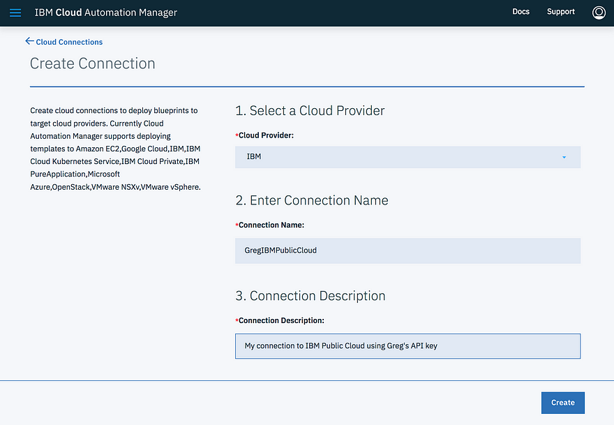
Figure 3: Select “Manage Connections” to create a new connection to IBM Cloud using your account to create the Kubernetes cluster.
This connection will use your IBM Cloud account’s API key to communicate between Cloud Automation Manager and IBM Cloud. Be aware that once you set this up, Cloud Automation Manager will use your account to create IBM Cloud resources. Be sure that your IBM Cloud account has the necessary user permissions and can support the billing for your estimated product usage.
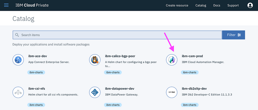
Third, create a custom service using an IBM-provided template to deploy an IBM Cloud Kubernetes Service cluster (with optional VPN connection) and publish it into the IBM Cloud Private catalog.
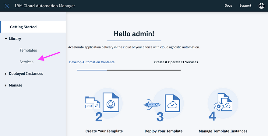
Figure 4: Select “Services” to create a new service in Cloud Automation Manager
This is really where you will harness the power of Cloud Automation Manager and its IBM-provided templates. Think of it this way: where in the past you would have to manually run commands or navigate a user interface to define the IBM Cloud Kubernetes Service, and then customize many details every time you provision a cluster, Cloud Automation Manager has provided all the details in a template. By creating this service, you provide a simple way to have your team provision a cluster when they need it, using the account (and limits) that you specify.
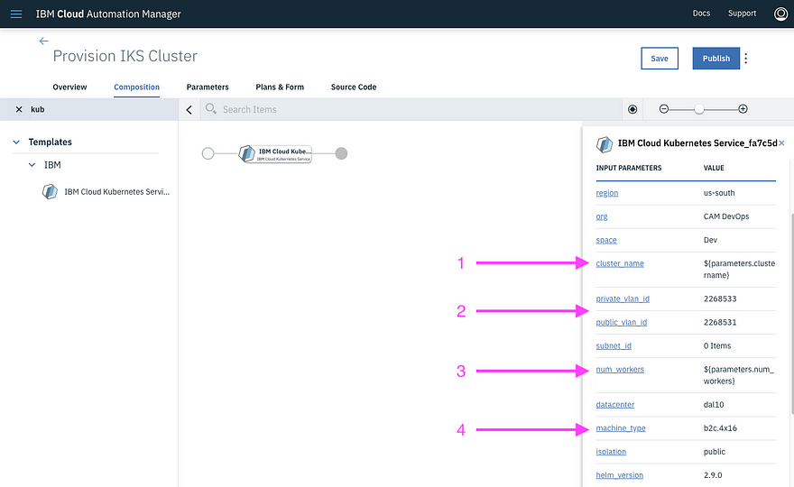
In addition to the previous link, here are some tips to creating the “Provision IKS Cluster” service (Figure 5):
Figure 5: Customizing parameters for your “Provision IKS Cluster” service
Make cluster_name a service parameter so your user can specify it when they deploy.
Specify private_vlan_id and public_vlan_id for the IBM Cloud region you want to deploy into. To find the values, run the following command in your IBM Cloud CLI (enter any location. In this example, ‘dal10’ is the location I want to deploy into): bx cs vlans dal10
Make num_workers (the number of worker nodes for the cluster) a service parameter so your users can decide how many worker nodes their cluster needs. Note that this should be an array of the number of workers you authorize your users to select from. Maybe start with offering 2–5 worker nodes.
Default machine_type so users can only select machines of the kind you default. To select your default, simply click the value column and all supported machine types will appear.
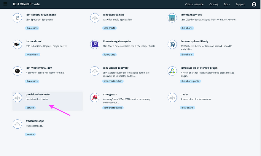
Once you publish the service into the IBM Cloud Private catalog, you will allow other users a simplified way to create their own clusters.
Figure 6: IBM Cloud Private catalog with the service to provision IKS cluster that you just created
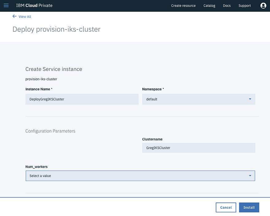
Fourth, deploy the “Provision IKS Cluster” service from the catalog. You’ll notice in Figure 7 that there are just a few parameters for the individual to fill out (the service you defined earlier filled in most of the defaults).
Figure 7: Deploying an IKS cluster from IBM Cloud Private
Now that your service is created, your development teams can deploy as many IBM Cloud Kubernetes Service clusters into the public cloud as they need.
Curate, to your enterprise standards, production services sourced from IBM Cloud Private and IBM Cloud Kubernetes Service into a single catalog.
The second enhancement is the ability to deploy production middleware into either IBM Cloud Private or IBM Cloud Kubernetes Service, all from your IBM Cloud Private catalog. This enhancement, coupled with the new IBM Cloud Private capability to limit what users have access to in the catalog, allows a cloud admin to give a developer a curated view of what they can deploy. Further, with IBM Cloud Automation Manager’s brokered service support, the cloud admin can create a service with multiple plans, so when a developer selects a plan in their catalog, IBM Cloud Automation Manager will deploy the proper version of middleware that maps to the selected plan.
For example, you may want to let a user “Create a database,” but without burdening them with all the specifics that a database Helm chart requires. Further, you have specific versions in mind, depending on where they deploy and who the user is. For instance, you may want to have only “dev” versions or “production” versions of the middleware on certain clusters, or even an open source Postgres database in IBM Cloud Kubernetes Service. With this new enhancement, you can create a brokered service through IBM Cloud Automation Manager to present a simplified view for the user to select their desired plan, hiding all the gritty details so that they can answer a few questions, deploy what they want, and you can manage the database instances far easier.
Here are the steps you will follow. For each step, I’ve added a link to the Knowledge Center that provides step-by-step instructions.
To import production middleware into IBM Cloud Kubernetes Service, you can either store the Helm charts in your local file system, or you can upload them into a private Helm repository. If you want to upload the charts into a private Helm repository, you will need to first deploy one into your cluster. IBM Cloud Kubernetes Service does not currently have a private Helm repository, so I recommend you install ChartMuseum, which will give you the needed private Helm repository in your IBM Cloud Kubernetes Service cluster.
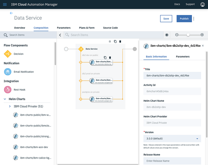
Third, open IBM Cloud Automation Manager in IBM Cloud Private to create the brokered database service, or whatever brokered service you want. As you did before, click “Create Service,” and this time, open “IBM Cloud Private,” which will show all the Helm charts you can add to this service.
Figure 8: Create a “Data Service” in Cloud Automation Manager
One concept that you need to know: Since the goal is to have one service deploy charts into either IBM Cloud Private or IBM Cloud Kubernetes Service, the list of Helm charts listed in IBM Cloud Automation Manager needs to be the union of Helm charts available in both targets. For you, this means that your IBM Cloud Private cluster needs to add the Helm repo URL of the IBM Cloud Kubernetes Service cluster so that the charts show up in this list.
Fourth, now that you have your customized service created, you can curate (filter, limit) what services show up for your developer, Jane. As you can see from the Cloud Automation Manager capabilities above, you can surface most any service from any cloud to your developers, customize and limit what parameters they can edit, and now with IBM Cloud Private 2.1.0.3, you can filter the catalog so Jane can only see what you want her to.
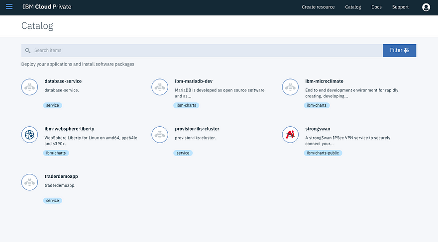
For example, while earlier in Figure 6 the admin has 54 items in the catalog, Figure 9 shows that Jane can see only seven!
Figure 9: Filtered catalog view for “Jane” the developer. Notice “Database-Service” and “Provision-IKS-Cluster”.
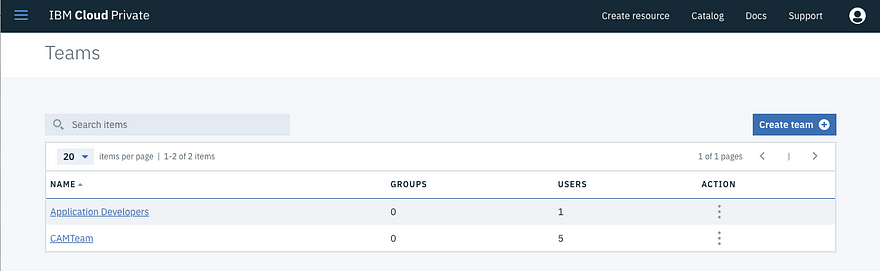
To filter the catalog, add a team like “Application Developers” in the Manage > Teams view (Figure 10).
Figure 10: Showing teams in IBM Cloud Private
Once created, click the team name, and the “Resources” tab. This will show all resources the team is authorized to. What I really like is that teams can be authorized to a variety of resources across IBM Cloud Private:
Kubernetes namespace (for increased isolation and access control)
Helm repo (so devs can access only the collection of Helm charts you want)
Individual Helm charts
Individual brokered services
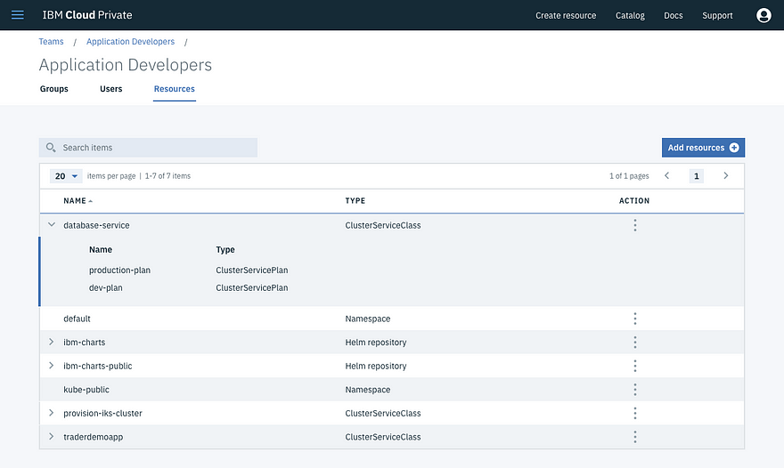
In Figure 11, you can see what application developers are authorized to. Notice that the database service we created previously has two plans, and the developers are authorized to both. However, you could authorize them to only one plan. This means that you could create one service and authorize portions to different teams…far easier to manage.
Figure 11: The resources available to application developers
Transform, develop, and deploy your application onto both IBM Cloud Private and IBM Cloud Kubernetes Service
The third enhancement revolves around helping developers migrate WebSphere apps and then deploying them into IBM Cloud Private using a pipeline to multiple Kubernetes clusters.
Here’s what you will need:
IBM Cloud Private
IBM Transformation Advisor
Microclimate
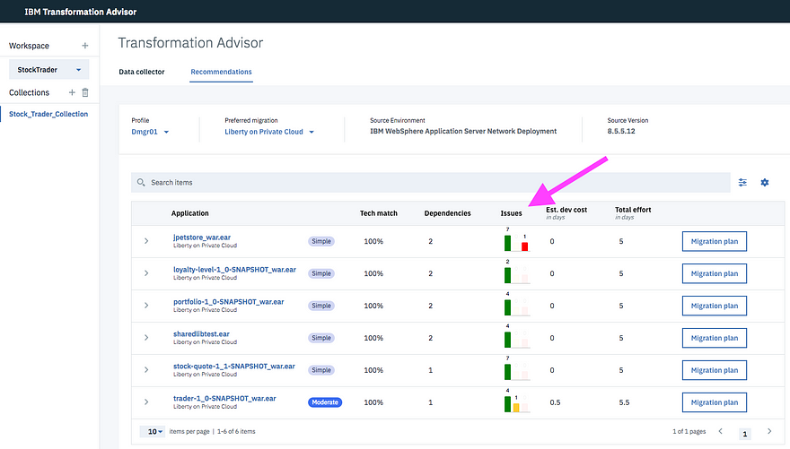
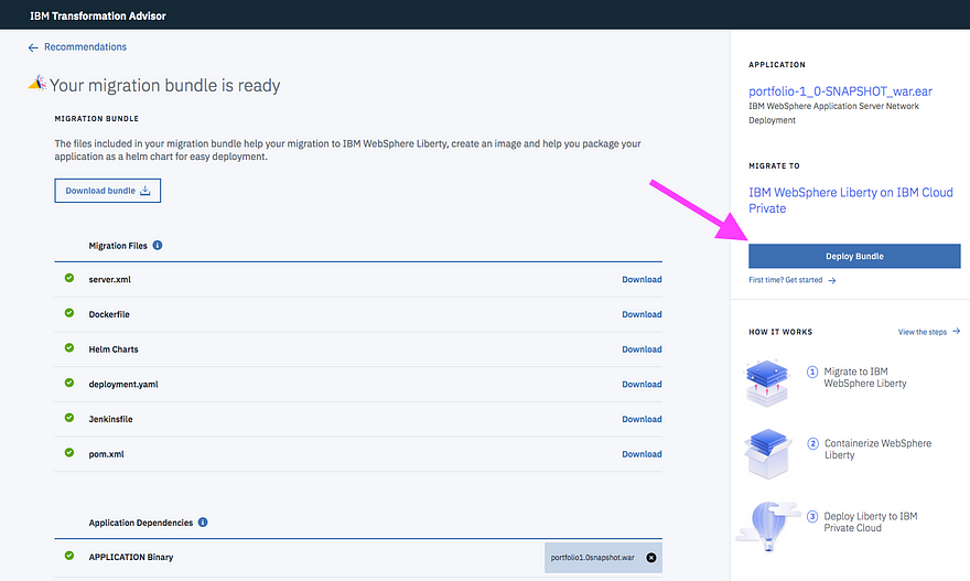
For example, to migrate a WebSphere application, start by running Transformation Advisor from your IBM Cloud Private instance. Transformation Advisor provides a data collector to add next to your WebSphere app, and it will provide recommendations on how to migrate it into a containerized WebSphere Liberty runtime on IBM Cloud Private.
In Figure 12, Transformation Advisor shows the results of its analysis. As you can see, each file is shown, the issues (how complicated it would be to migrate), and a migration plan.
Figure 12: The resources available to application developers
In the migration plan for each file (Figure 13), Transformation Advisor shows all the deployment files it would create and provides a link to deploy the bundle.
Figure 13: The detailed migration plan for a specific bundle
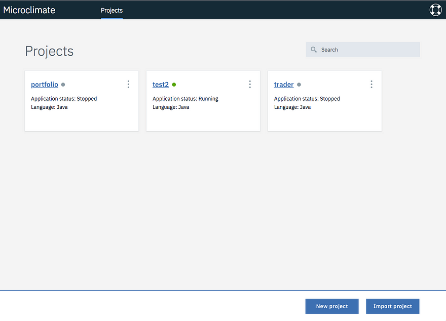
Figure 14 shows Microclimate and the projects that were created:
Figure 14: Microclimate and its projects
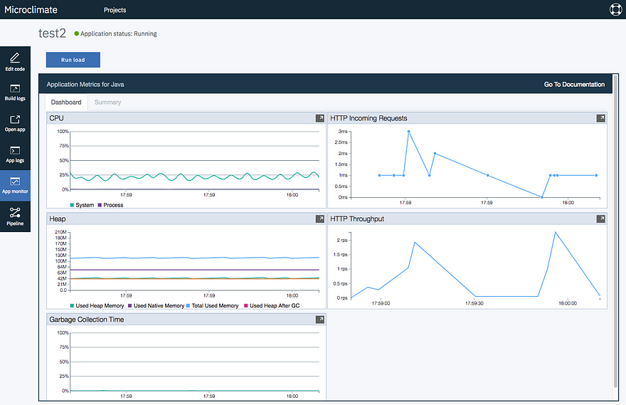
Once you select a project that you imported, you could update the Git repo with source code and soon you can update code, view logs, and even view app-level metrics like in Figure 15:
Figure 15: Coding and unit testing apps all within Microclimate
Finally, to deploy the app to additional clusters (like a remote IBM Cloud Private or IBM Cloud Kubernetes Service), you can set up deployment pipelines additional clusters using these instructions.
Summary
As you can see, if you need to run your app in a hybrid environment that makes it easier for developers to provision services they need (wherever they may reside), and if your developers need faster ability to deploy across multiple Kubernetes clusters, these enhancements will be quite welcome since now, with IBM Cloud Private 2.1.0.3, Fix Pack 1, users can:
Create additional Kubernetes clusters using a template from IBM Cloud Private
Curate which services developers have access to, and let them provision on either private or public clusters with self-service capability
Deploy a custom app into both private and public environments from the same developer environment
I hope you give this a try, and if you need any help, contact IBM Cloud Private support here: http://ibm.biz/icpsupport
One of my greatest joys at IBM is showing customers how they can use IBM solutions to solve problems and improve their business. A common problem we hear is that enterprise clients need to run their apps locally, while leveraging the value of the cloud. In general they want to keep sensitive data local while integrating cloud benefits such as rapid deployment, continuous delivery, and microservices, and they want this to include Java applications.
Recently we released IBM Cloud private, a Kubernetes-based private cloud, which runs in your data center. You can start small, manage it yourself, and grow it to run whatever workloads you want. IBM Cloud private provides key runtimes and services that you depend on, such as Liberty, Db2, MQ, Microservice Builder, Redis, and much more. (learn more here).
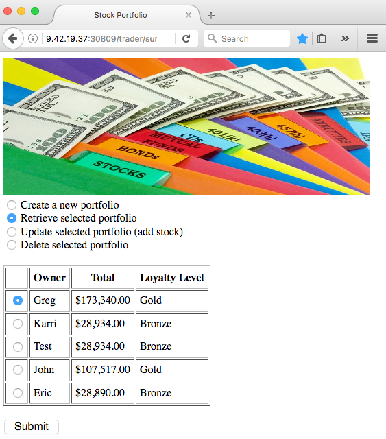
In this article, I will show how we stood up our private cloud, and used this private cloud to deploy a stock trader application. This stock trader application is a Java microservices app that is running in Liberty, uses Db2, MQ, and Redis, and can also connect to a public cloud.
Here is a quick video summarizing what we built that will provide context for the rest of this article.
My hope is that you can repeat our success by following what we did, and if you have any questions, feel free to join the conversation in the comments.
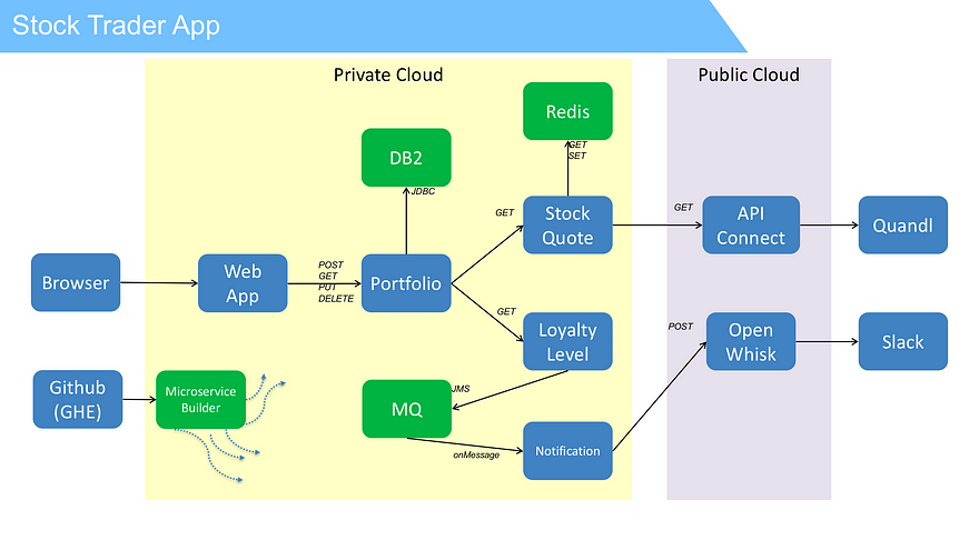
The Architecture
We set out to develop a stock trader application that would run using local data, yet connect to the public cloud to get stock quotes and post messages when a customer’s loyalty level changed….a true Hybrid solution. We needed a database, a messaging queue, and a local cache. We also wanted the ability to continuously make code changes and update only what was needed. The result was an application architecture shown in Figure 1.
Figure 1: Application architecture including GitHub Enterprise and Microservice Builder to support continuous delivery goals
With that in mind, we then architected what our private cloud should look like. The results of this is shown in Figure 2.
Figure 2: Cloud layout, including DSM to help manage the database, and four VMs to run our cloud.
I cannot stress enough how important this layout step is. As you will see, there is a lot of communication that is required between the developer and the cloud administrator. The alignment between app and cloud architecture is essential to ensure that the solution meets the need of both parties.
The Plan
Our plan was straight-forward:
Set up IBM Cloud private
Set up the services that we needed
Add secrets to improve developer productivity
Run the application in IBM Cloud private
Integrate with Microservice Builder
Continuously deliver!
To truly understand what our clients would experience, we decided to role-play the personas we were designing for: Todd the cloud admin, and Jane the enterprise developer. In the end, this was a fantastic way to ensure that we could realistically prepare all aspects of the stock trader solution.
Setting Up IBM Cloud private
The first thing we did was set up IBM Cloud private. We followed the detailed instructions here. We got pretty good at it so now we can do it in about 1.5 hours. As you follow these instructions, here are a couple of tips:
Use the same node as both Master and Boot.
When you set up your SSH keys across your nodes, run the commands from the master node to itself.
If your VMs are running on different subnets, add the following line to your config.yaml:
calico_ipip_enabled: true
Once the IBM Cloud private environment was installed, we took a breath and opened the IBM Cloud private UI (Figure 3).
Figure 3: Manage the apps, storage, network, and compute nodes from this operations UI.
Figure 4: Kubernetes Dashboard UI, an opensource UI provided by Kubernetes
Our next step was to install each service that we needed: Db2, MQ, and Redis.
Seting Up Services
When I talked with our developer, we wanted to incrementally move into IBM Cloud private. Why? Well, there are many variables so if we could just try one thing, make it work, then try the next thing, we ended up achieving our goal faster than setting up the whole solution and hope it “just worked”.
For example, we wanted to test out the services before he moved his application into IBM Cloud private. Kubernetes nicely supports that by offering two ways to network into a service: Internally through “ClusterIP”, and externally through the proxy server using “NodePort”. Take a look at our MQ service in Figure 5:
Figure 5: the `kubectl describe` command showing service details
You will see an internal port 1414 only accessible inside the Kubernetes cluster by using the default-mq-mq:1414, and a NodePort 31966 that is available outside the private cloud using proxyNodeIPaddress:31966.
As a result, our developer could access MQ from his running code (basically changing one variable) and we could confirm that the services worked great. Then, once the app was using all services from the developer’s workstation, we added secrets and moved his app inside the private cloud.
OK, now we actually set up the services.
Setting Up DB2
Thanks to a handy recipe, installing DB2 was easy:
Once Db2 was running, we had to prime the database with the tables that the app needed.
Since Db2 installs automatically with a database called ‘sample’. We then added a ‘Stock’ and ‘Portfolio’ table to this database. We also added a configuration option that automatically deleted all rows in the Stock table that referenced deleted row in the Portfolio table. That way, the code didn’t have to iterate over each stock for a portfolio and delete it, prior to deleting the portfolio itself.
These are the commands we ran. We could have run this command from the DB2 command line: “db2 -tf createTables.ddl” but we installed DSM, so we ran these as SQL statements in DSM:
CREATE TABLE Portfolio(owner VARCHAR(32) NOT NULL, total DOUBLE, loyalty VARCHAR(8), PRIMARY KEY(owner));
CREATE TABLE Stock(owner VARCHAR(32) NOT NULL, symbol VARCHAR(8) NOT NULL, shares INTEGER, price DOUBLE, total DOUBLE, dateQuoted DATE, FOREIGN KEY (owner) REFERENCES Portfolio(owner) ON DELETE CASCADE, PRIMARY KEY(owner, symbol));
To verify it’s all working, we connected DSM to our DB2 database (Figure 6)
Figure 6: DSM lets you monitor multiple databases, run SQL statements, and view the database content through the Administer menu.
We could also verify that our Db2 setup is successful by running the following SQL statement:
SELECT * FROM Employee
Eventually, once our stock trader app was running, we replaced Employee, a table in the Sample database, with Portfolio, our table with our private data.
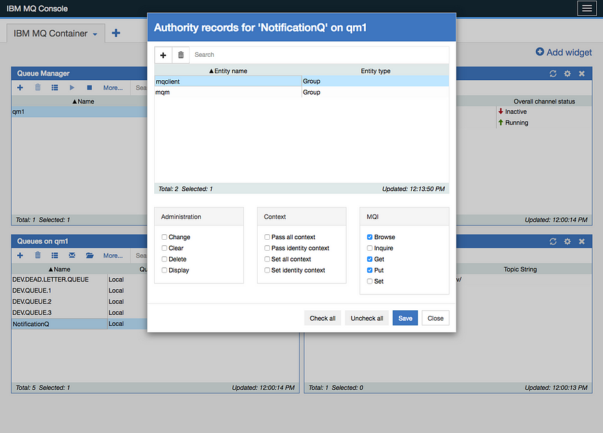
Once MQ was running, we needed to create the message queue that the app expected. I logged into the MQ UI and created a queue called, ‘NotificationQ’ (Figure 7)
Figure 7: Create the NotificationQ
Next, we had to authorize the app user ID ‘app’ to the queue. The MQ instructions said NOT to use the default admin ID, but to use the default application ID, ‘app’.
When you add ‘app’, it will show the group name as ‘mqclient’. From the MQI section, select the Browse, Get, and Put options (Figure 8).
Figure 8: ‘mqclient’ was added with the correct authority to browse, get, and put.
Setting Up Redis
To set up redis, we used the Redis app located in the IBM Cloud private App Center.
First, log into the IBM Cloud private UI: https://masternodeIP:8443/#/dashboard/ with the default user ID and password set to admin/admin. Once logged in, select the left menu and then “App Center”. Find Redis, and install it.
Setting Up API Connect and Quandl
As you’ve seen in past blogs, this stock trader app is built from earlier editions that use API Connect in IBM’s public cloud to then call Quandl. This version does not require API Connect, but if you want to learn more, and read how we’re calling Quandl to get stock quotes, read about it here.
Setting Up OpenWhisk and Slack Messaging
Another capability we built from previous editions of the stock trader application was to call an OpenWhisk action that sends a slack message. To get that portion working, you’ll want to read about it here.
Creating secrets
We have a recipe describing why secrets are so useful, and you can read it here. In a nutshell they make your application portable by letting you define custom, cloud-specific information regarding how the app can use each service.
Here are the secrets that we created for our stock trader application.
MQ Secret
First, we found the MQ service name
kubectl get svc
Then viewed the properties
kubectl describe service default-mq-mq
If you set up the services with NodePort, two ports will appear for internal and external access to the application. And another two ports for the UI. By default, port 1414 is what the application uses when the app is running inside the private cloud.
This Redis secret should actually be called, “the stock quote microservice secret” because it contains details to access Redis, as well as details to access Quandl, a provider of stock quotes. We found we could call Quandl 50 times per day without registering, or if we registered (no cost), it bumped that up to 300 calls per day (To register for Quandl, see http://quandl.com/ ).
We ran this to find the Redis service name
kubectl get svc
Then viewed the properties
kubectl describe service worn-horse-redis
To create the secret that the application can use, we needed to get the Redis password secret that the Redis install already created, and then add it into the secret our developer would use. Here’s what we used to set a password parameter in Kubernetes:
Finally, we created this secret (using the password parameter, service name, port, and our quandl key. If you don’t want to register, just leave the quandl-key field empty):
At this point, we decided to test the application inside IBM Cloud private (and you can too). Why? Because our code was in Eclipse on our developer’s laptop, and it was the next incremental step to build containers and then deploy them into IBM Cloud private. For us, it was a whole additional set of variables to move our code into GitHub and connect to our private cloud through Microservice Builder that we were not ready for yet (We’ll walk through how to do that next)
The proxy IP is the IP address of the VM acting as proxy node. The ‘traderPort’ is the external NodePort, and can be found using the same commands as above.
We ran this to find the Redis service name
kubectl get svc
Then viewed the properties
kubectl describe service trader-service
Make sure you use the NodePort, usually in the 30000 range.
Integrating with Microservice Builder
You may be asking, “I have the app running now, why bother with Microservice Builder”? For us, while it was tedious to set up Microservice Builder, we found that integrating with Microservice Builder saved us an amazing amount of time!
If you want to continuously deliver and enhance your app’s micro-services, you should use Microservice Builder. Our experience was that whenever we wanted to tweak a behavior, we could just change the code in GitHub, commit the changes, and…PRESTO, Microservice Builder would detect the changes, build them, and deploy updated containers into our private cloud.(Figure 9 and 10).
Figure 9: Micro-services are being built
Figure 10: Microservices are built successfully.
To start, follow the instructions to install Microservice Builder here. Read it closely. There are many manual steps around authenticating the Microservice Builder pipeline with GitHub that you need to pay attention to:
To be honest, we followed these instructions and still had problems. Here are a few tips that might help to reduce these problems for you:
Make the GitHub repos public. Microservice Builder does not work with private repositories.
Configure IBM Cloud private so that pods can access the private Docker image registry when deploying. We missed the fact in the article and took quite some time to realize it.
Add your entire team as “admins” when setting up Microservice Builder. We found it was difficult to add people after deployment.
In section 4 of the steps, the instructions mentions adding single quotes around the “Master.JavaOpts” field setting. Don’t do that. This instruction is old (it’s being updated, but not changed yet). Just keep it as it is.
Finally, if you are going to try Microservice Builder with your own code, here are some tips:
Use Maven to build. We had experience with Gradle, so needed to switch to Maven.
Using the command “bx dev” added the proper files to your GitHub repo so Microservice Builder knows what to do with the code.
Move your deployment.yaml into the manifest folder.
Stock Trader In Action — Through Microservices
Now lets take a peek at how we found value with all of this running. You can refer back to Figure 1 to see the application architecture. Here’s a screen shot of the trader web UI (Figure 11)
Figure 11: Stock trader app rendered from the ‘trader’ micro-service
From a web browser we connected to the “trader” micro-service that renders the simple web app. While it’s quite basic, we did want to change a few things and since it is a small micro-service, we could redeploy updates to the “trader” UI in seconds. Further, since Kubernetes handled the networking, we didn’t have to worry about changing IP addresses or DNS changes ourselves.
Another big time-saver was using the Liberty “Datasource” in the portfolio micro-service. This allowed us to switch out completely different databases (even switch between DB2, Oracle, sqlServer, etc.). All we had to do was update the db2 secret, restart portfolio, and it connected where we wanted to
As you add stock to a portfolio, the Stock Quote micro-service is contacted. It checks Redis to see if there is a local cache that is within 24 hours old, and if not, connects to quandl.com to fetch the latest stock quote. Once the portfolio is updated, the Loyalty Level micro-service is contacted which calculates if the user has reached the next level. In this case the Loyalty Level microservice determines I’ve achieved “Gold” level, so it sends a message to MQ.
As soon as the message is added to NotificationQ, the “Notification” micro-service notices it, calls OpenWhisk to trigger a message in our Slack channel. This is a great example of how a private cloud app can utilize a public cloud service while the sensitive data (the portfolio details) stays local.
Summary
We learned so much building this stock trader application. I encourage you to try it yourself, or even parts of it. In addition to the video overview, take advantage of the recipes (Db2, MQ, Secrets), and if you want to run our stock trader app (or fork it and start making changes), access it here: